Quantum capacitance¶

Example¶

The function simple.GrapheneQuantumCapacitance() illustrates the usage of the quantum capacitance solver:

def GrapheneQuantumCapacitance():
    """
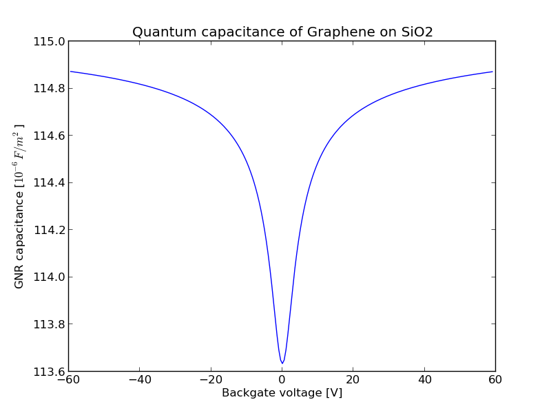
    Calculate the quantum capacitance of Graphene on SiO2, including temperature.

    Boundary conditions:

    * left, right: periodic BC
    * top: Neumann BC, slope=0
    * bottom: backgate capacitor plate

    Please read the code comments for further documentation.

    """
    #Set system parameters
    gridsize=1e-9
    hoehe=600
    breite=1
    backgatevoltage=0
    graphenepos=299
    temperature=300
    sio2=3.9

    vstart=-60
    vend=60
    dv=0.5

    #Finite difference operator
    lapl=electrostatics.Laplacian2D2ndOrderWithMaterials(gridsize,gridsize)
    #Create Rectangle
    periodicrect=electrostatics.Rectangle(hoehe,breite,1.,lapl)

    #Set boundary condition at the top
    for y in range(breite):
        periodicrect[0,y].neumannbc=(0,'xf')

    #Create list of backgate and GNR elements
    backgateelements=[periodicrect[hoehe-1,y] for y in range(breite)]
    grapheneelements=[periodicrect[graphenepos,y] for y in range(breite)]

    #Set initial backgate element boundary condition (not necessary)
    for element in backgateelements:
        element.potential=backgatevoltage

    #Create D(E,T) function
    Ef_dependence_function=quantumcapacitance.BulkGrapheneWithTemperature(temperature,gridsize).Ef_interp

    #Set electrochemical potential and D(E,T) for the GNR elements
    for element in grapheneelements:
        element.potential=0
        element.fermi_energy=0
        element.fermi_energy_charge_dependence=Ef_dependence_function

    #Set dielectric material
    for x in range(graphenepos,hoehe):
        for y in range(breite):
            periodicrect[x,y].epsilon=sio2

    #Create periodic container
    percont=electrostatics.PeriodicContainer(periodicrect,'y')

    #Invert discretization matrix
    solver,inhomogeneity=percont.lu_solver()

    #Create QuantumCapacitanceSolver object
    qcsolver=quantumcapacitance.QuantumCapacitanceSolver(percont,solver,grapheneelements,lapl)

    #Refresh basisvectors for calculation. Necessary once at the beginning.
    qcsolver.refresh_basisvecs()

    #Create volgate list
    voltages=numpy.arange(vstart,vend,dv)

    charges=[]

    #Loop over voltages
    for v in voltages:
        #Set backgate elements to voltage
        for elem in backgateelements:
            elem.potential=v
        #Check change of environment
        qcsolver.refresh_environment_contrib()
        #Solve quantum capacitance problem & set potential property of elements
        qcsolution=qcsolver.solve()
        #Create new inhomogeneity because potential has changed
        inhom=percont.createinhomogeneity()
        #Solve system with new inhomogeneity
        sol=solver(inhom)
        #Save the charge configuration in the GNR
        charges.append(percont.charge(sol,lapl,grapheneelements))
    #Sum over charge and take derivative = capacitance
    totalcharge=numpy.array([sum(x) for x in charges])
    capacitance=(totalcharge[2:]-totalcharge[:-2])/len(grapheneelements)*gridsize/(2*dv)

    #Plot result
    fig=pylab.figure()
    ax = fig.add_subplot(111)
    ax.set_title('Quantum capacitance of Graphene on SiO2')
    ax.set_xlabel('Backgate voltage [V]')
    ax.set_ylabel('GNR capacitance [$10^{-6} F/m^2$]')
    pylab.plot(voltages[1:-1],1e6*capacitance)

The result:

Code reference¶

class envtb.quantumcapacitance.quantumcapacitance.BulkGrapheneWithTemperature(T, grid_height, interpolation=True)[source]¶

How the Fermi energy of graphene (Dirac cone) depends on the charge density at finite temperatures.

The algorithm includes a function inversion, which can either be done with interpolation (Ef_interp()) or with a root search (Ef()). The interpolation is strongly suggested for higher speed.

If you use Q() often, you should probably also implement an interpolation to improve speed.

The variables minEf, max Ef, Eftol, dEf are the parameters for the interpolation/root search. minEf and maxEf have to span the relevant energy window around the equilibrium Fermi energy = 0. If steps occur, decrease Eftol/dEf.

Check Ef() if it’s still working properly!!!

You will probably use Q() as charge_fermi_energy_dependence and Ef() or Ef_interp() as fermi_energy_charge_dependence.

If you don’t want to use Ef_interp(), you can set interpolation=False.

static FermiEnergyChargeDependence.bulk_graphene(charge, grid_height=1e-09)[source]¶

How the Fermi energy of graphene depends on the charge density at 0K.

class envtb.quantumcapacitance.quantumcapacitance.QuantumCapacitanceSolver(container, solver, elements, charge_operator, equation='potential', nonlocal_charge_potential_function=None)[source]¶

Calculates the quantum capacitance of a system with a density of states D(E). D(E,x) should work too (with equation=’charge_nonlocal), but hasn’t been tested yet.

Note: QuantumCapacitanceSolver changes the potential property of the participating elements. The constant property is fermi_energy (i.e. if you connect an external voltage of 5V, set fermi_energy=5).

Usage:

1. Create object: qcsolver=QuantumCapacitanceSolver(container,solver, elements,operator)
2. Calculate classical dependency of charge on every possible potential configuration of elements: qcsolver.refresh_basisvecs()
3. Set potential/fermi_energy as you like (e.g. backgate, sidegates...).
4. Refresh the contribution of the new configuration: qcsolver.refresh_environment_contrib()
5. Solve: qcsolution=qcsolver.solve()
6. go to 3) until you are through with all voltages you want to look at.

container: the container which describes the system. solver: the solution of the system, e.g. generated by my_container.lu_solver(). elements: the elements (from the system described by container) that participate in the calculation. The property fermi_energy_charge_dependence needs to be set. charge_operator: The operator which gives the charge (without epsilon_0). equation: there are three formulations of the problem: ‘charge’,’potential’ and ‘charge_nonlocal’.

Default is ‘potential’. For ‘charge’, the element’s charge_fermi_energy_dependence property is used. For ‘potential’, the element’s fermi_energy_charge_dependence property is used. You don’t have to set the property that you don’t use. For ‘charge_nonlocal’, you only have to provide the nonlocal_charge_potential_function

nonlocal_charge_potential_function: use together with equation=’charge_nonlocal’.

Mind to calculate the volume charge density, not the area charge density! The argument will be the difference vector Fermi_energy(x)-potential(x).